Links for this session

Google Colab notebook
Materials for this session
Source notebook
Local data file used in this post: data/niamey.csv
Example of final output
PDF version of materials (with code and outputs)

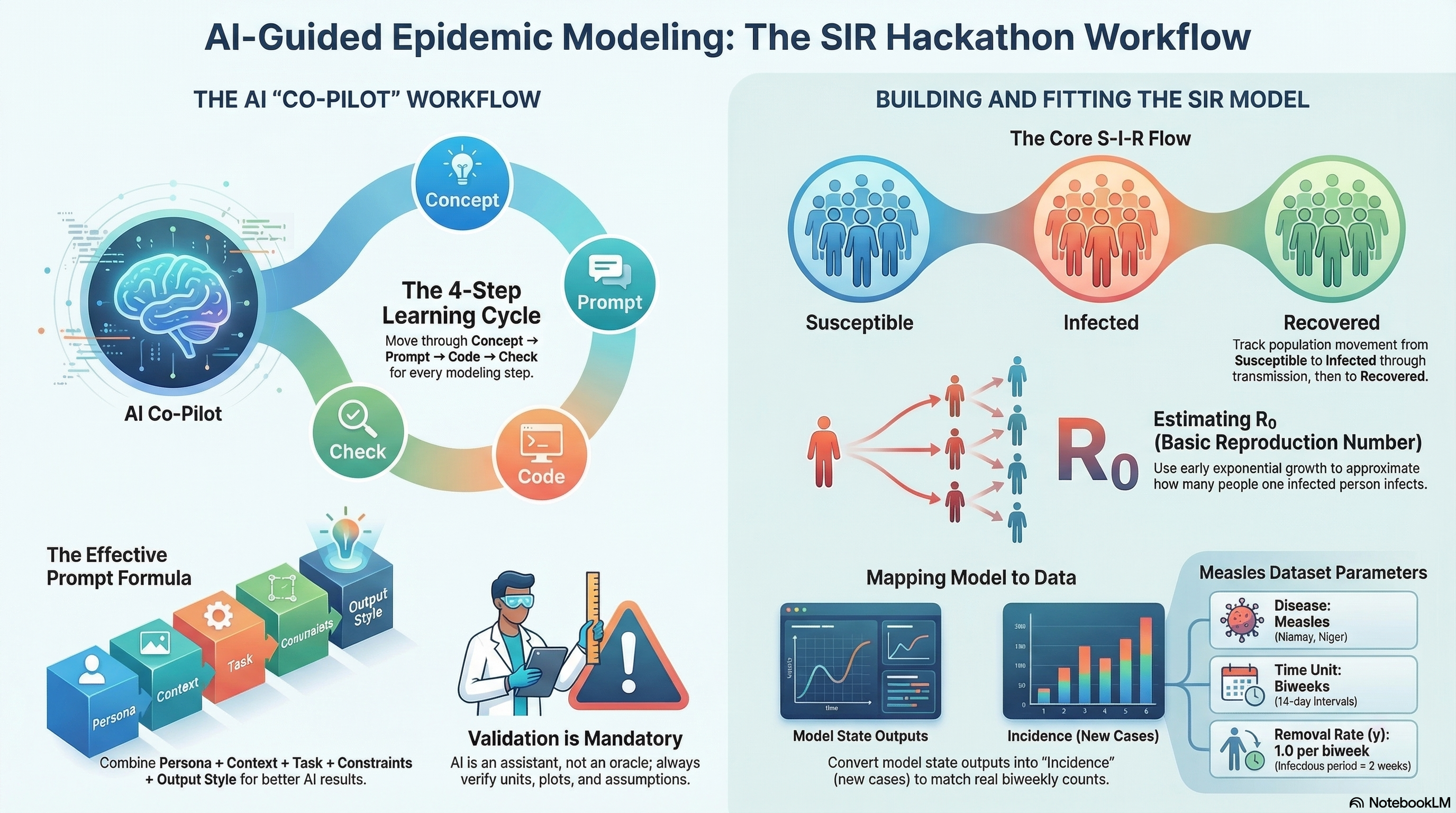
AI-Guided SIR Modeling Hackathon (2 Hours)

This notebook is the workshop skeleton for the AI-Guided SIR Modeling Hackathon.

Dataset: Niamey, Niger measles outbreaks (biweekly case counts; communities A/B/C)
Tooling: Google Colab + Python + ChatGPT
Time unit: biweeks
Key modeling shortcut: infectious period ≈ 2 weeks ⇒ γ ≈ 1 per biweek

Overview

This live session uses prompt-driven analysis to move from raw biweekly measles counts to a calibrated SIR model for Community A.

By the end of the session, participants should be able to:

Explore incidence patterns in data/niamey.csv
Estimate early outbreak growth and approximate R0
Map SIR model output to observed incidence via cumulative infections
Fit model parameters with least squares and Poisson likelihood
Interpret uncertainty using a simple profile likelihood

Before the session

Open the Colab notebook linked above.
Confirm the dataset path is data/niamey.csv (relative path).
Make sure Python can import numpy, pandas, scipy, and matplotlib.
Review the workflow sections below so you know where each prompt fits.

What is Google Colab?

Google Colab (short for “Colaboratory”) is a free, browser-based notebook environment where you can run Python code without installing a local Python setup.

For this session, Colab helps you:

Run the workshop notebook directly from a shared link
Execute code in small cells and inspect outputs step-by-step
Combine narrative text, prompts, code, and figures in one place
Save your own copy in Google Drive for continued practice

Tips for first-time users:

Use Runtime > Run all to execute all cells in order
If a cell fails, read the error, fix the prompt/code, then rerun that cell
If the runtime disconnects, reconnect and rerun from the top

Troubleshooting

Common issues and quick fixes

FileNotFoundError: verify you are using the relative path data/niamey.csv.
Missing package errors: install/import numpy, pandas, scipy, and matplotlib.
Flat or unstable fits: revise the selected early biweek window and re-run prompts.
Predicted vs observed mismatch: confirm incidence alignment (t[1:] vs delta_H) in prompt logic.
Log-scale confusion: ensure you only log-transform strictly positive case counts.

Resources

How to use this notebook

Each section contains: 1) A ChatGPT prompt (Markdown) you can copy into ChatGPT
2) A starter code cell (often with TODOs) to run in Colab

Rule of thumb: Always request plots + sanity checks when you ask ChatGPT for help.

0. Setup

ChatGPT Prompt (copy/paste)

Persona:
You are an expert epidemiological modeler and Python educator.

Task:
- Write a Colab-ready setup cell: imports, basic plotting config, and a helper for reproducibility.
- If any package is missing show me how to run pip install

Constraints:
- Use numpy, scipy, pandas, matplotlib only

Verification:
- Print library versions and a simple "ready" message.

1. Explore the Niamey Measles Data:

Load the dataset and compute basic statistics

ChatGPT Prompt (copy/paste)

Persona:
You are an expert epidemiological modeler and Python educator.

Context:
- Dataset contains biweekly measles case counts from Niamey, Niger
- File path: data/niamey.csv

Task:
Write Python code to:
1. Load data/niamey.csv store it to `measles_df`
2. Display the first few rows
3. Print column names and basic information about the dataset
4. Show basic statistics about dataset

Constraints
- Use pandas only
- Keep code simple and readable

Exercise

TODO: Participants write a prompt to explain the results in plain language

Basic Plot

ChatGPT Prompt (copy/paste)

Persona:
You are an expert epidemiological modeler and Python educator.

Context:
- Dataset is already loaded into a DataFrame called `measles_df`
- Columns: biweek, community, measles

Task:
- Plot measles cases over time for each community
- Use one time-series plot
- Label axes and include a legend
- Briefly explain what biweekly case counts mean for epidemic modeling

2. Feature-Based Estimation: Early Growth (Quick R₀)

We estimate early exponential growth using a semi-log regression: - Choose an early window where cases grow roughly exponentially. - Fit log(cases) vs time.

ChatGPT Prompt (copy/paste)

## Persona

You are an **expert in infectious disease modeling**, with experience in early-outbreak analysis and interpretation of epidemic growth rates.

## Context

* **Disease:** Measles
* **Community:** A
* **Data:** Biweekly reported case counts
* **Epidemic phase:** Early outbreak (first ~8–10 biweeks), where case counts exhibit **exponential growth**
* **Dataset:** Already loaded as `measles_df`

### Dataset structure

`
<class 'pandas.core.frame.DataFrame'>
RangeIndex: 48 entries, 0 to 47
Columns:
- biweek     (int64)
- community  (object)
- measles    (float64, 47 non-null)
`

## Task

Estimate the **early exponential growth rate** of the outbreak by:

1. Selecting an appropriate **early biweek window** (≈ 8–10 biweeks)
2. Fitting a **log-linear model**: log(measles cases) vs. time
3. Producing a **semi-log plot** showing observed data and fitted exponential growth
4. Converting the estimated growth rate to an **approximate basic reproduction number (R₀)**, assuming:

   * Infectious removal rate: **γ = 1 per biweek**

## Constraints

* Use **NumPy** and **SciPy** only (Matplotlib for plotting is acceptable)
* Clearly **state and explain modeling assumptions**
* Print key **statistical results** (e.g., slope, confidence intervals if available, R₀)
* **Output code only** (do not execute)

## Verification / Expected Output

* A **semi-log plot** of measles cases with the fitted exponential curve
* Printed values for:

  * Estimated **growth rate (slope)**
  * Corresponding **R₀ estimate**

Goal Assess how sensitive the estimated basic reproduction number (R₀) is to the choice of early-outbreak window length.

Method (brief) For a sequence of increasing early-outbreak windows (measured in biweeks):

Fit a log-linear model to early reported measles cases to estimate the exponential growth rate.
Convert the growth rate to R₀ assuming a fixed infectious removal rate (γ = 1 per biweek).
Compute a 95% confidence interval for R₀ from the regression uncertainty.
Visualize R₀ and its uncertainty as a function of the window length.

Interpretation Stable R₀ estimates across window lengths suggest a robust early-growth signal, while strong variation indicates sensitivity to window choice or departures from exponential growth.

Continue with the the prompt

For a range of early-outbreak window lengths, plot the estimated R₀ (derived from exponential growth rates) together with its 95% confidence interval, as a function of the initial period length (in biweeks).

3. Implement the SIR Model (Biweekly Units)

We use a closed SIR model for a single outbreak wave: - S(t): susceptible - I(t): infectious - R(t): recovered

Time unit = biweeks.

ChatGPT Prompt (copy/paste)

Persona:
You are an expert epidemiological modeler and Python educator.

Context:
- Closed SIR model (no birth or death)
- Time unit: biweeks
- Infectious period ≈ 2 weeks (gamma ≈ 1 per biweek)

Task:
Implement an SIR model using SciPy ODE solving:
- Define the SIR equations, the function name should be `sir_rhs`
- Solve over a biweekly time grid, put it in the function `simulate_sir`
- Plot S, I, R over time

Constraints:
- Use scipy.integrate.solve_ivp
- Keep code readable and commented

Verification:
- Plot S, I, R
- Verify S + I + R ≈ N

4. Map Model Output to Observations (Incidence via ΔH)

Observed data are biweekly case counts, not the state I(t).
We model incidence using an accumulator:

Add H(t) with dH/dt = β S I / N
Predicted biweekly counts ≈ ΔH over each biweek interval

ChatGPT Prompt

Persona:
You are an expert epidemic modeler.

Context:
- Observed data are biweekly case counts (incidence)
- SIR model outputs states

Task:
Extend the SIR model by:
- Adding H(t) with dH/dt = beta*S*I/N
- Computing predicted biweekly cases as ΔH aligned to biweeks

Constraints:
- Keep code minimal and readable

Verification:
- Plot predicted ΔH

Continue with the prompt to plot the data

I have biweekly measles incidence data for Community A:

measles_df = pd.read_csv("data/niamey.csv")

dfA = (
    measles_df
    .loc[measles_df["community"] == "A", ["biweek", "measles"]]
    .dropna(subset=["measles"])
    .copy()
)

- dfA["biweek"] contains the biweekly time index

- dfA["measles"] contains observed biweekly incidence (number of cases)

I also have an SIR model that returns simulated incidence:

def simulate_sir_with_incidence(
    N=1000,
    I0=1,
    R0=0,
    beta=2.5,
    gamma=1.0,
    t_max=20
):
    ...
    return t, S, I, R, H, delta_H

Where:

t → model time points (in biweeks)

delta_H → simulated biweekly incidence (new infections per biweek)

H → cumulative infections

What I want to do

- Plot observed measles incidence (dfA["measles"])

- Overlay simulated biweekly incidence (delta_H) on the same figure

- Use t[1:] when plotting delta_H as len(t) is different from len(delta_h) by 1 unit

5. Fit Parameters by Least Squares

We fit parameters by minimizing squared error between observed counts and predicted ΔH.

ChatGPT Prompt (copy/paste)

## 👤 Persona

You are an **expert in numerical optimization for epidemic models**, with experience fitting compartmental models to incidence data using nonlinear least squares.

---

## 📂 Data

We have **biweekly measles incidence data** for **Community A**:

measles_df = pd.read_csv("data/niamey.csv")

dfA = (
    measles_df
    .loc[measles_df["community"] == "A", ["biweek", "measles"]]
    .dropna(subset=["measles"])
    .copy()
)

* `dfA["biweek"]` → biweekly time index
* `dfA["measles"]` → observed biweekly incidence (case counts)

---

##  Model

We use an SIR model that returns simulated incidence:

def simulate_sir_with_incidence(
    N=1000,
    I0=1,
    R0=0,
    beta=2.5,
    gamma=1.0,
    t_max=20
):
    ...
    return t, S, I, R, H, delta_H

Where:

* `t` → model time points (in biweeks)
* `delta_H` → simulated **biweekly incidence** (new infections per biweek)
* Use `t[1:]` to align with `delta_H` (since incidence is computed between time steps)

---

## 🎯 Objective

Fit model parameters to the observed incidence data using **nonlinear least squares**.

### Parameters to estimate:

* `N` (population size)
* `beta` (transmission rate)
* Optional: `I0` (initial infected)

### Fixed parameter:

* `gamma = 1.0`

---

## 📈 Initialization Strategy

Use an early-growth estimate:

* Estimated basic reproduction number:

  [
  R_0 = 1.443
  ]

* Since ( R_0 = \beta / \gamma ), initialize:

  [
  \beta_0 = 1.443
  ]

Choose reasonable initial guesses and bounds:

* `N` within plausible community size range
* `beta > 0`
* `I0 ≥ 1`

---

## ⚙️ Optimization Requirements

* Use `scipy.optimize.least_squares`
* Fit by minimizing:

[
\text{SSE} = \sum ( \text{Observed} - \text{Predicted} )^2
]

* Ensure runtime is suitable for a workshop (avoid heavy MCMC or expensive methods)

---

## 📊 Verification & Output

After fitting:

1. Overlay observed and fitted incidence curves
2. Print:

   * Best-fit parameter values
   * Sum of squared errors (SSE)

---

## 📌 Expected Deliverables

* Residual function definition
* Call to `least_squares`
* Overlay plot (observed vs fitted)
* Printed parameter estimates and SSE
* Clean, reproducible workshop-ready code

6. Poisson Likelihood Inference (Counts)

For count data: - ( y_t (_t) ) - ( _t = H_t )

where ρ is a reporting/ascertainment fraction.

ChatGPT Prompt (copy/paste)

# 👤 Persona

You are an **expert in numerical optimization for epidemic models**, with experience fitting compartmental models to incidence data using likelihood-based methods.

---

# 📂 Data

We have **biweekly measles incidence data** for **Community A**:

measles_df = pd.read_csv("data/niamey.csv")

dfA = (
    measles_df
    .loc[measles_df["community"] == "A", ["biweek", "measles"]]
    .dropna(subset=["measles"])
    .copy()
)

t_obs = dfA["biweek"].values
y_obs = dfA["measles"].values

* `t_obs` → biweekly time index
* `y_obs` → observed biweekly incidence (case counts)

---

#  Model

We use an SIR model that returns simulated incidence:

def simulate_sir_with_incidence(
    N=1000,
    I0=1,
    R0=0,
    beta=2.5,
    gamma=1.0,
    t_max=20
):
    ...
    return t, S, I, R, H, delta_H

Where:

* `t` → model time points (in biweeks)
* `delta_H` → simulated **biweekly incidence**
* Use `t[1:]` to align with `delta_H`

---

# 🎯 Objective

Fit model parameters to the observed incidence data using **maximum likelihood under a Poisson observation model**.

Assume:

[
Y_t \sim \text{Poisson}(\lambda_t)
]

where:

* ( Y_t ) = observed incidence
* ( \lambda_t ) = model-predicted incidence (`delta_H`)

---

# 📌 Parameters to Estimate

* `N` (population size)
* `beta` (transmission rate)
* Optional: `I0` (initial infected)

### Fixed parameter:

* `gamma = 1.0`

---

# 📈 Initialization Strategy

Use early-growth estimate:

[
R_0 = 1.443
]

Since:

[
R_0 = \beta / \gamma
]

Initialize:

[
\beta_0 = 1.443
]

Use reasonable bounds:

* `N` within plausible community size range
* `beta > 0`
* `I0 ≥ 1`

---

# ⚙️ Optimization Requirements

Use `scipy.optimize.minimize` (or `least_squares` minimizing −log-likelihood).

Minimize the **negative Poisson log-likelihood**:

[
\mathcal{L}(\theta)
===================

\sum_t \left(
\lambda_t - y_t \log(\lambda_t)
\right)
]

(omit constant (\log(y_t!)) term)

Add small epsilon to avoid `log(0)`.

Ensure runtime is suitable for a workshop (no MCMC).

---

# 📊 Verification & Output

After fitting:

1. Overlay observed and fitted incidence curves
2. Print:

   * Best-fit parameter values
   * Final negative log-likelihood
3. (Optional) Compare visually against least-squares fit

---

# 📌 Expected Deliverables

* Negative log-likelihood function definition
* Call to optimizer
* Overlay plot (observed vs fitted incidence)
* Printed parameter estimates
* Clean, reproducible workshop-ready code
* Proper numerical safeguards (`epsilon` for stability)

7. Quick Uncertainty: Profile Likelihood for β (Optional)

ChatGPT Prompt (copy/paste, continue with the likelihood chat)

Persona:
You are an expert in likelihood-based inference.

Context:
- We already have a Poisson likelihood fit
- We want uncertainty for beta

Task:
Create a profile likelihood for beta:
1) Fix beta over a grid
2) Optimize I0 and rho for each beta
3) Plot profile NLL(beta)

Constraints:
- Keep runtime reasonable for a workshop

Verification:
- Profile plot
- Explain how to interpret the uncertainty

Live Session 8: AI-Guided SIR Modeling Hackathon

AI-Guided SIR Modeling Hackathon (2 Hours)

Overview

Before the session

What is Google Colab?

Troubleshooting

Resources

How to use this notebook

0. Setup

ChatGPT Prompt (copy/paste)

1. Explore the Niamey Measles Data:

Load the dataset and compute basic statistics

ChatGPT Prompt (copy/paste)

Exercise

Basic Plot

ChatGPT Prompt (copy/paste)

2. Feature-Based Estimation: Early Growth (Quick R₀)

ChatGPT Prompt (copy/paste)

Continue with the the prompt

3. Implement the SIR Model (Biweekly Units)

ChatGPT Prompt (copy/paste)

4. Map Model Output to Observations (Incidence via ΔH)

ChatGPT Prompt

5. Fit Parameters by Least Squares

ChatGPT Prompt (copy/paste)

6. Poisson Likelihood Inference (Counts)

ChatGPT Prompt (copy/paste)

7. Quick Uncertainty: Profile Likelihood for β (Optional)

ChatGPT Prompt (copy/paste, continue with the likelihood chat)

8. Generate a Markdown Summary (Hackathon Report Cell)

ChatGPT Prompt (copy/paste)