# (Optionnel) Installer les packages si nécessaire
# install.packages(c("sf", "tmap", "ggspatial", "ggrepel", "tidyverse"))
# remotes::install_github("malaria-atlas-project/malariaAtlas")Introduction
Ce document consiste a faire de la cartographie avec des commentaires en français.
Pré-requis : R ≥ 4.2, et les packages
sf,tmap,ggspatial,ggrepel,tidyverse,malariaAtlas.
Téléchargement des données
# Télécharger et décompresser les données (AMMnet Hackathon)
url <- "https://raw.githubusercontent.com/AMMnet/AMMnet-Hackathon/main/03_mapping-r/data.zip"
download.file(url, "data.zip", mode = "wb")
unzip("data.zip", exdir = ".")
Chargement des bibliothèques
library(sf)
library(tmap)
library(ggspatial)
library(ggrepel)
library(tidyverse)
library(malariaAtlas)
Données spatiales : polygones et points
# Importer le shapefile des régions (Admin1) de Tanzanie
tz_admin1 <- st_read("data/shapefiles/TZ_admin1.shp", quiet = TRUE)
tz_admin1
Simple feature collection with 36 features and 16 fields
Geometry type: MULTIPOLYGON
Dimension: XY
Bounding box: xmin: 29.3414 ymin: -11.7612 xmax: 40.4432 ymax: -0.9844
Geodetic CRS: WGS 84
First 10 features:
iso admn_lv name_0 id_0 type_0 name_1 id_1 type_1
1 TZA 1 Tanzania 10001003 Country Arusha 10316307 Region
2 TZA 1 Tanzania 10001003 Country Morogoro 10313017 Region
3 TZA 1 Tanzania 10001003 Country Lake Tanganyika 604100824 Water Body
4 TZA 1 Tanzania 10001003 Country Lake Victoria 604100823 Water Body
5 TZA 1 Tanzania 10001003 Country Lindi 10313079 Region
6 TZA 1 Tanzania 10001003 Country Manyara 10313760 Region
7 TZA 1 Tanzania 10001003 Country Mara 10314956 Region
8 TZA 1 Tanzania 10001003 Country Mbeya 10314026 Region
9 TZA 1 Tanzania 10001003 Country Mjini Magharibi 10313694 Region
10 TZA 1 Tanzania 10001003 Country Mtwara 10316433 Region
name_2 id_2 type_2 name_3 id_3 type_3 source cntry_l
1 NA NA NA NA NA NA Tanzania NBS 2020 TZA_1
2 NA NA NA NA NA NA Tanzania NBS 2020 TZA_1
3 NA NA NA NA NA NA Tanzania NBS 2020 TZA_1
4 NA NA NA NA NA NA Tanzania NBS 2020 TZA_1
5 NA NA NA NA NA NA Tanzania NBS 2020 TZA_1
6 NA NA NA NA NA NA Tanzania NBS 2020 TZA_1
7 NA NA NA NA NA NA Tanzania NBS 2020 TZA_1
8 NA NA NA NA NA NA Tanzania NBS 2020 TZA_1
9 NA NA NA NA NA NA Tanzania NBS 2020 TZA_1
10 NA NA NA NA NA NA Tanzania NBS 2020 TZA_1
geometry
1 MULTIPOLYGON (((35.2613 -1....
2 MULTIPOLYGON (((38.2698 -6....
3 MULTIPOLYGON (((31.2069 -8....
4 MULTIPOLYGON (((31.7822 -0....
5 MULTIPOLYGON (((39.5821 -9....
6 MULTIPOLYGON (((35.3626 -3....
7 MULTIPOLYGON (((33.3328 -2....
8 MULTIPOLYGON (((33.031 -6.8...
9 MULTIPOLYGON (((39.3401 -6....
10 MULTIPOLYGON (((40.4279 -10...# Charger les données ponctuelles PfPR (MIS Tanzanie 2017)
tz_pr <- readr::read_csv("data/pfpr-mis-tanzania-clean.csv", show_col_types = FALSE)
head(tz_pr)# A tibble: 6 × 27
id country country_id continent site_id site_name latitude longitude
<dbl> <chr> <chr> <chr> <dbl> <chr> <dbl> <dbl>
1 1071935 Tanzania TZA Africa 1071933 TZ2017000002… -3.68 33.4
2 1071947 Tanzania TZA Africa 1071945 TZ2017000002… -3.64 33.4
3 1071737 Tanzania TZA Africa 1071735 TZ2017000002… -5.22 31.7
4 1071041 Tanzania TZA Africa 1071039 TZ2017000000… -8.61 38.8
5 1072997 Tanzania TZA Africa 1072995 TZ2017000004… -6.14 39.2
6 1072811 Tanzania TZA Africa 1072809 TZ2017000003… -2.99 31.9
# ℹ 19 more variables: rural_urban <chr>, month_start <dbl>, year_start <dbl>,
# month_end <dbl>, year_end <dbl>, lower_age <dbl>, upper_age <dbl>,
# examined <dbl>, pf_pos <dbl>, pf_pr <dbl>, method <chr>, rdt_type <chr>,
# pcr_type <lgl>, dhs_id <chr>, source_id1 <dbl>, source_id2 <dbl>,
# source_id3 <lgl>, date <date>, survey_type <chr># Convertir les points en objet 'sf' (WGS84)
tz_pr_points <- st_as_sf(tz_pr, coords = c("longitude", "latitude"), crs = 4326)
tz_pr_pointsSimple feature collection with 436 features and 25 fields
Geometry type: POINT
Dimension: XY
Bounding box: xmin: 29.65546 ymin: -11.38231 xmax: 40.30508 ymax: -1.124763
Geodetic CRS: WGS 84
# A tibble: 436 × 26
id country country_id continent site_id site_name rural_urban month_start
* <dbl> <chr> <chr> <chr> <dbl> <chr> <chr> <dbl>
1 1.07e6 Tanzan… TZA Africa 1071933 TZ201700… URBAN 10
2 1.07e6 Tanzan… TZA Africa 1071945 TZ201700… URBAN 10
3 1.07e6 Tanzan… TZA Africa 1071735 TZ201700… RURAL 10
4 1.07e6 Tanzan… TZA Africa 1071039 TZ201700… RURAL 10
5 1.07e6 Tanzan… TZA Africa 1072995 TZ201700… URBAN 10
6 1.07e6 Tanzan… TZA Africa 1072809 TZ201700… URBAN 10
7 1.07e6 Tanzan… TZA Africa 1071759 TZ201700… RURAL 10
8 1.07e6 Tanzan… TZA Africa 1072563 TZ201700… RURAL 10
9 1.07e6 Tanzan… TZA Africa 1071303 TZ201700… RURAL 10
10 1.07e6 Tanzan… TZA Africa 1072581 TZ201700… RURAL 10
# ℹ 426 more rows
# ℹ 18 more variables: year_start <dbl>, month_end <dbl>, year_end <dbl>,
# lower_age <dbl>, upper_age <dbl>, examined <dbl>, pf_pos <dbl>,
# pf_pr <dbl>, method <chr>, rdt_type <chr>, pcr_type <lgl>, dhs_id <chr>,
# source_id1 <dbl>, source_id2 <dbl>, source_id3 <lgl>, date <date>,
# survey_type <chr>, geometry <POINT [°]>Premières cartes avec ggplot2
# Carte simple des régions
ggplot(tz_admin1) +
  geom_sf() +
  theme_bw() +
  labs(title = "Régions de Tanzanie")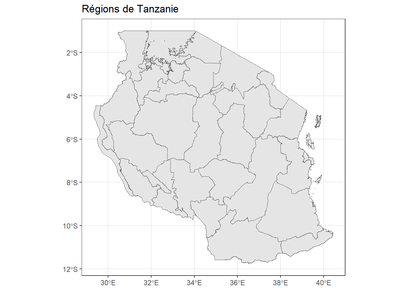
# Carte régions + points PfPR (données data.frame)
ggplot() +
  geom_sf(tz_admin1, mapping = aes(geometry = geometry)) +
  geom_point(tz_pr, mapping = aes(x = longitude, y = latitude, color = pf_pr)) +
  scale_color_distiller(palette = "Spectral") +
  theme_bw() +
  labs(color = "PfPR, 0–5 ans")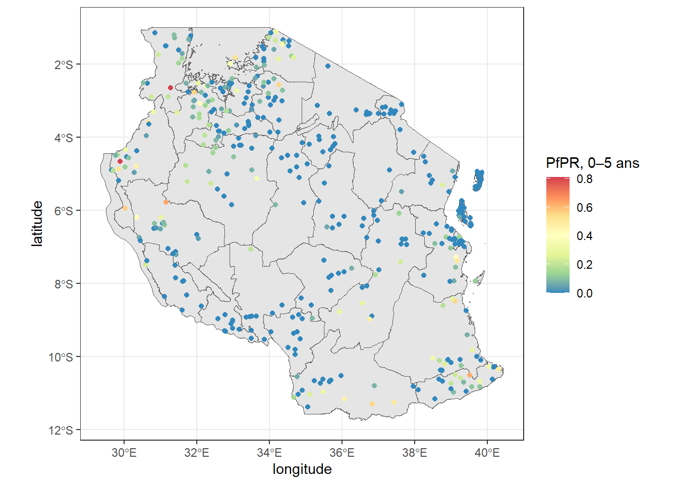
# Carte régions + points PfPR (objets sf uniquement)
ggplot() +
  geom_sf(tz_admin1, mapping = aes(geometry = geometry)) +
  geom_sf(tz_pr_points, mapping = aes(geometry = geometry, color = pf_pr)) +
  scale_color_distiller(palette = "Spectral") +
  theme_minimal() +
  labs(title = "Prévalence du paludisme 0–5 ans — MIS Tanzanie 2017",
       color = "PfPR")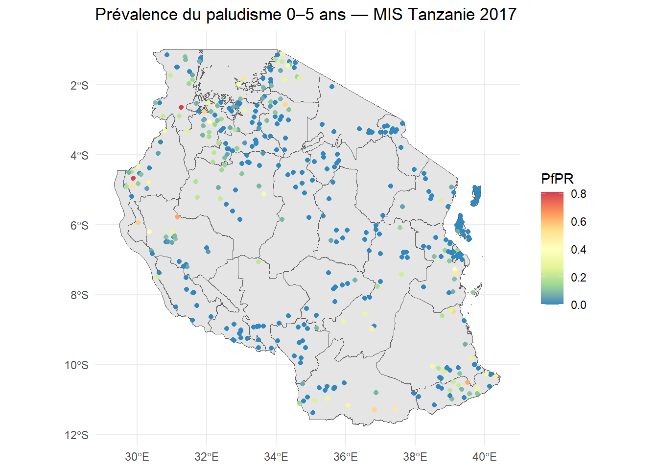
Jointure des données de population (Admin1)
OBJECTIF :
Charger la table de population Admin1, harmoniser les noms de régions pour qu’ils correspondent à ceux du shapefile (tz_admin1), puis vérifier la concordance avant de joindre les données.
# 1) Charger la population Admin1 depuis un CSV (affichage des types désactivé)
tz_pop_adm1 <- readr::read_csv("data/tza_admpop_adm1_2020_v2.csv", show_col_types = FALSE)

# 2) Harmoniser les noms pour correspondre au shapefile
#    - str_to_title() met les noms en « Titre » (première lettre en majuscule)
#    - case_when() corrige manuellement les divergences connues entre sources
tz_pop_adm1 <- tz_pop_adm1 %>%
  dplyr::mutate(name_1 = stringr::str_to_title(ADM1_EN)) %>%
  dplyr::mutate(
    name_1 = dplyr::case_when(
      name_1 == "Dar Es Salaam" ~ "Dar-es-salaam",
      name_1 == "Pemba North" ~ "Kaskazini Pemba",
      name_1 == "Pemba South" ~ "Kusini Pemba",
      name_1 == "Zanzibar North" ~ "Kaskazini Unguja",
      name_1 == "Zanzibar Central/South" ~ "Kusini Unguja",
      name_1 == "Zanzibar Urban/West" ~ "Mjini Magharibi",
      name_1 == "Coast" ~ "Pwani",
      TRUE ~ as.character(name_1)  # conserver les autres noms tels quels
    )
  )

# 3) Vérifier la concordance des noms entre le shapefile (tz_admin1$name_1)
#    et la table de population harmonisée (tz_pop_adm1$name_1)
#    - TRUE = correspondance trouvée ; FALSE = pas de correspondance
table(tz_admin1$name_1 %in% tz_pop_adm1$name_1)
FALSE  TRUE
    5    31
# (Optionnel) Lister explicitement les noms du shapefile non retrouvés dans la population
# unmatched <- setdiff(tz_admin1$name_1, tz_pop_adm1$name_1)
# if (length(unmatched)) {
# message("Noms non appariés (shapefile → population) :")
# print(unmatched)
# }
# (Étape suivante typique, non incluse ici) :
# tz_pop_admin1 <- tz_admin1 %>% dplyr::left_join(tz_pop_adm1, by = "name_1")# Joindre population au shapefile
tz_pop_admin1 <- tz_admin1 %>% left_join(tz_pop_adm1, by = "name_1")# Carte de population totale (lacs en bleu clair, transformation racine)
ggplot(tz_pop_admin1) +
geom_sf(mapping = aes(fill = T_TL)) +
scale_fill_viridis_c(option = "B", na.value = "lightblue", trans = "sqrt") +
theme_bw() +
labs(title = "Population en Tanzanie (2020)",
fill = "Population totale")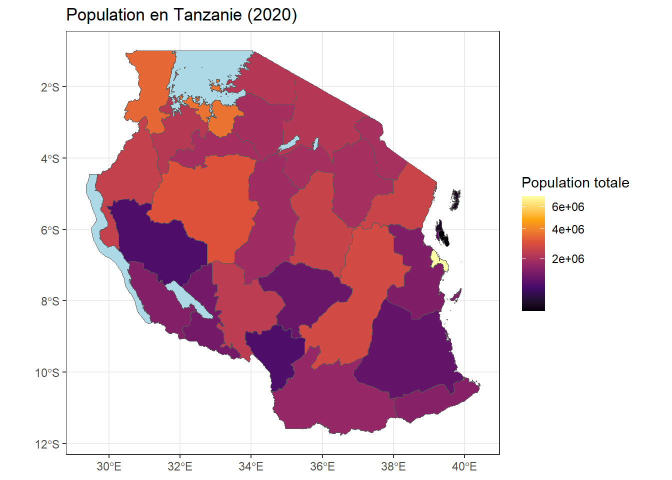
Attribution régionale des points PfPR et agrégation
# Désactive la géométrie sphérique 's2' et repasse sur GEOS (plan)
# Utile quand certaines opérations de jointure/validation échouent avec s2
# (ex. géométries invalides, buffers en degrés, incohérences topologiques).
# ⚠️ Pense à éventuellement réactiver plus tard : sf_use_s2(TRUE)
sf_use_s2(FALSE)

# Jointure spatiale : pour chaque POINT de tz_pr_points, on récupère
# l'attribut du POLYGONE (tz_admin1) qui le contient.
# Par défaut, le prédicat est st_intersects (point-dans-polygone).
# Résultat : un sf de points enrichi des colonnes de tz_admin1 (dont name_1).
tz_pr_point_region <- st_join(tz_pr_points, tz_admin1)

# Agrégation par région :
tz_region_map <- tz_pr_point_region %>%
  ungroup() %>%                 # s'assurer qu'aucun groupement antérieur n'est actif
  group_by(name_1) %>%          # regrouper tous les points par nom de région (Admin1)
  summarise(
    # moyenne non pondérée du PfPR par région ;
    # si besoin, remplacer par une moyenne pondérée (taille d'échantillon, population, etc.)
    mean_pr = mean(pf_pr, na.rm = TRUE)
  ) %>%
  st_drop_geometry() %>%        # on retire la géométrie des points (on garde un data.frame agrégé)
  # Rejoindre la table agrégée aux polygones pour obtenir un objet sf polygonal
  # contenant la colonne 'mean_pr' par région.
  left_join(tz_admin1, ., by = "name_1")
# Carte de PfPR moyen par région
ggplot(tz_region_map) +
geom_sf(mapping = aes(fill = mean_pr)) +
scale_fill_distiller(palette = "Spectral", na.value = "lightblue") +
theme_bw() +
labs(fill = "PfPR moyen, 0–5 ans",
title = "Prévalence par région en Tanzanie",
subtitle = "MIS 2017")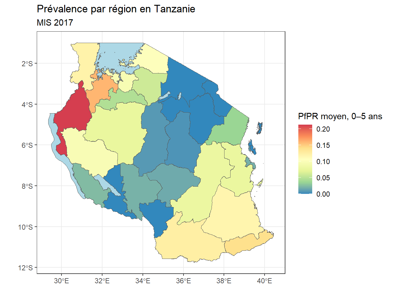
Tampons (buffers) et projections
# Créer un buffer ~20 km autour des points (≈ 0,2° près de l’équateur)
tz_pf_buffer_20km <- st_buffer(tz_pr_points, dist = 0.2)

ggplot(tz_admin1) +
  geom_sf() +
  geom_sf(tz_pf_buffer_20km, mapping = aes(geometry = geometry), alpha = 0.2) +
  geom_sf(tz_pr_points, mapping = aes(color = pf_pr), size = 0.6) +
  scale_color_distiller(palette = "Spectral") +
  labs(color = "PfPR, 0–5 ans", subtitle = "MIS 2017") +
  theme_minimal()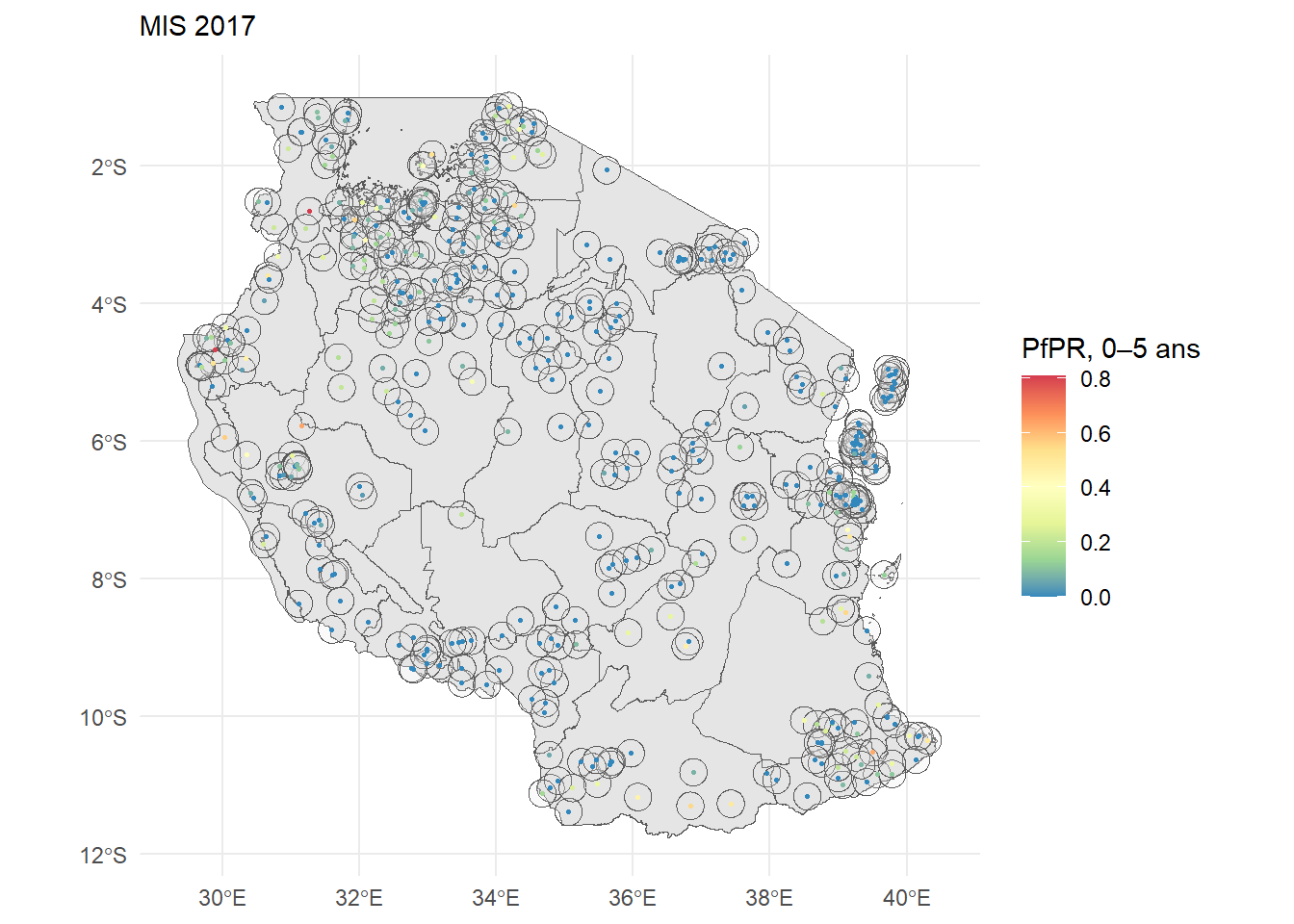
# Vérifier / changer la projection (UTM zone 35S, EPSG:32735)
st_crs(tz_admin1)
Coordinate Reference System:
User input: WGS 84
wkt:
GEOGCRS["WGS 84",
DATUM["World Geodetic System 1984",
ELLIPSOID["WGS 84",6378137,298.257223563,
LENGTHUNIT["metre",1]]],
PRIMEM["Greenwich",0,
ANGLEUNIT["degree",0.0174532925199433]],
CS[ellipsoidal,2],
AXIS["latitude",north,
ORDER[1],
ANGLEUNIT["degree",0.0174532925199433]],
AXIS["longitude",east,
ORDER[2],
ANGLEUNIT["degree",0.0174532925199433]],
ID["EPSG",4326]]st_crs(tz_pr_points)Coordinate Reference System:
User input: EPSG:4326
wkt:
GEOGCRS["WGS 84",
ENSEMBLE["World Geodetic System 1984 ensemble",
MEMBER["World Geodetic System 1984 (Transit)"],
MEMBER["World Geodetic System 1984 (G730)"],
MEMBER["World Geodetic System 1984 (G873)"],
MEMBER["World Geodetic System 1984 (G1150)"],
MEMBER["World Geodetic System 1984 (G1674)"],
MEMBER["World Geodetic System 1984 (G1762)"],
MEMBER["World Geodetic System 1984 (G2139)"],
MEMBER["World Geodetic System 1984 (G2296)"],
ELLIPSOID["WGS 84",6378137,298.257223563,
LENGTHUNIT["metre",1]],
ENSEMBLEACCURACY[2.0]],
PRIMEM["Greenwich",0,
ANGLEUNIT["degree",0.0174532925199433]],
CS[ellipsoidal,2],
AXIS["geodetic latitude (Lat)",north,
ORDER[1],
ANGLEUNIT["degree",0.0174532925199433]],
AXIS["geodetic longitude (Lon)",east,
ORDER[2],
ANGLEUNIT["degree",0.0174532925199433]],
USAGE[
SCOPE["Horizontal component of 3D system."],
AREA["World."],
BBOX[-90,-180,90,180]],
ID["EPSG",4326]]tz_admin1_utm <- st_transform(tz_admin1, 32735)
tz_pr_points_utm <- st_transform(tz_pr_points, 32735)Carte « prête pour publication »
# Ajouter flèche du nord et barre d’échelle
publication_pr_map <- ggplot(tz_region_map) +
  geom_sf(mapping = aes(fill = mean_pr)) +
  scale_fill_distiller(palette = "Spectral", na.value = "lightblue") +
  annotation_north_arrow(location = "tr", height = unit(0.5, "cm"), width = unit(0.5, "cm")) +
  annotation_scale(location = "bl") +
  theme_void() +
  labs(fill = "PfPR moyen, 0–5 ans",
       title = "Prévalence par région en Tanzanie",
       subtitle = "MIS 2017")

publication_pr_map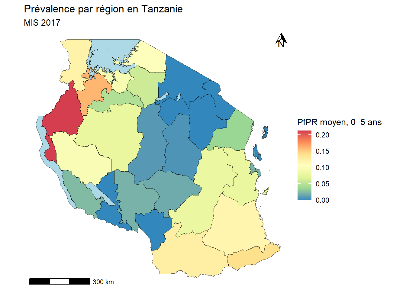
# (Optionnel) Ajouter les noms de régions
publication_pr_map +
  geom_sf_text(mapping = aes(label = name_1), size = 1.5)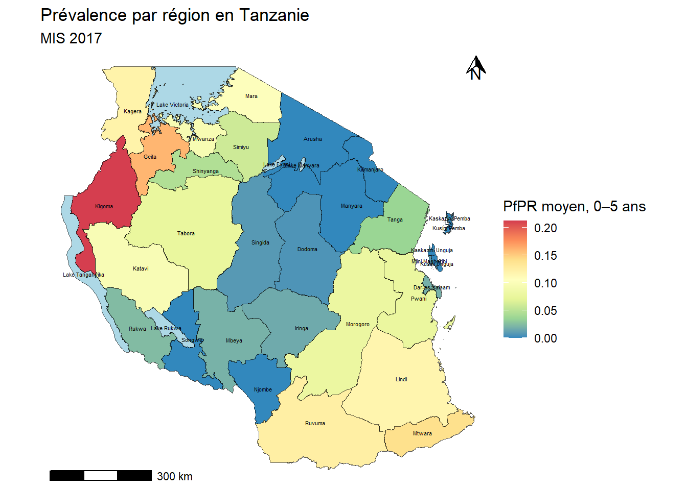
Export des résultats
# Exporter la figure et un shapefile exemple
#ggsave(filename = "tanzania_pr_map_2017.png", plot = publication_pr_map, width = 8, height = 6, dpi = 300)

# Shapefile population enrichie
#st_write(tz_pop_admin1, "data/shapefiles/tz_population_admin1.shp", delete_layer = TRUE)

# Shapefile des seules régions
tz_region_only <- dplyr::filter(tz_admin1, type_1 == "Region")
#st_write(tz_region_only, "data/shapefiles/tz_regions_only.shp", delete_layer = TRUE)
Cartes interactives (tmap)
# Polygones simples
tm_shape(tz_admin1) + tm_polygons()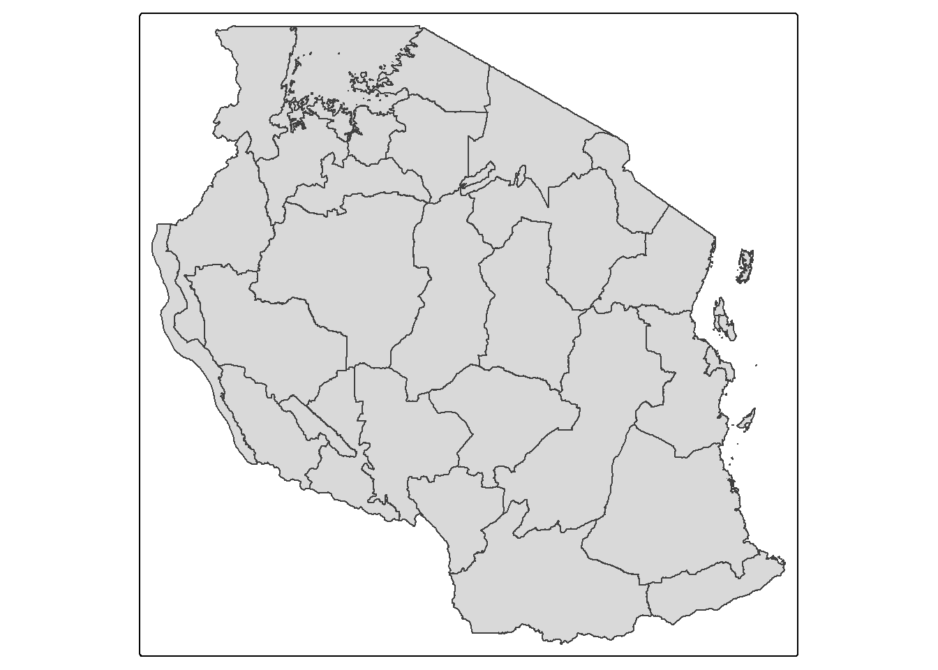
# Carte population avec palette viridis (classes 'pretty')
tm_shape(tz_pop_admin1) +
  tm_polygons("T_TL",
              palette = "viridis",
              title   = "Population",
              style   = "pretty", n = 4,
              colorNA = "lightblue", textNA = "lacs") +
  tm_layout(legend.outside = TRUE)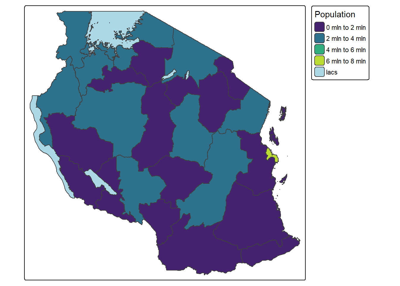
# Mode interactif
tmap_mode("view")

tm_shape(tz_pop_admin1) +
  tm_polygons("T_TL",
              id      = "name_1",   # étiquette interactive par région
              palette = "viridis",
              title   = "Population",
              style   = "pretty", n = 4,
              colorNA = "lightblue", textNA = "lacs") +
  tm_layout(legend.outside = TRUE)